On the technical debt of high-performance scientific software
High-performance scientific software must overcome two specific challenges: scientific validation, and performance on bleeding-edge and short-lived hardware. Success in each requires time, a high level of expertise, and the accumulated experience of many failed attempts. This explains why software developers in the field of engineering are mostly experts in physical modelling or in high-performance computing (HPC), however almost none are experts in the management of technical debt.
Technical debt is the implied cost of additional rework caused by choosing an easy (limited) solution now instead of using a better approach that would take longer (Wikipedia).
Once the code exists, just keeping up with the new ever more complex configurations or new HPC architecture, and often both, is a never-ending critical task. As a consequence, mainstream software challenges, such as scaling up to a high number of users or ensuring a good user experience, are far from being critical.
This is why high-performance scientific software developers are concerned about technical debt, but cannot put it at the top of their list of priorities.
The EXCELLERAT CoE cares a lot about technical debt because it is the key to transforming high-potential HPC codes into high added-value tools for engineering design. So how bad is the situation?

A primer on the DNA of a software code: the codebase
The codebase of any software is the collection of human-written source code. The software executable is built on any machine from this unique codebase. In a way, the codebase is to a code what DNA is to a human.
The codebase is like a book written for both computers (to execute the action) and humans (to understand the action). Here is a sample:
ifld = 2
if(ifflow) ifld = 1
do iel = 1,nelv
do ifc = 1,2*ndim
boundaryID(ifc,iel) = bc(5,ifc,iel,ifld)
enddo
enddo
Nek5000/src/connect2.f l113-119. Expressed in an Excel way, this snippet copies a subset of the sheet bc in a smaller sheet boundaryID, with iel the row ids. and ifc the column ids.
To understand this sample, one must know the language (here Fortran) and the context (what is behind these strange names such as ifflow). In all aspects it is like reading a book. The usual readers here are the Nek5000 developers’ community.
Several contributors add, change or delete lines in the book. The stream of changes is irregular, with occasional “bursts” of additions (many lines added) followed by heaps of very small changes. One can get a good mental image of this with the animations of gource.
A codebase rendered by the gource project, where developers look like bees building their home.
The AVBP gource animation highlights the high number of concurrent developers working simultaneously on the same codebase. All these additions and deletions are safely recorded in a Version Control System (VCS). For scientific HPC applications, rich in failed attempts painfully corrected, the exhaustive history of stored VCS is a priceless knowledge base.
Mining information from the history of real codebases
Here we will use some of the techniques in Your Code as a Crime Scene written by Adam Tornhill, a programmer who has specialized in code quality since 2010.
The codes under analysis are AVBP and Nek5000, two core CFD solvers that are part of EXCELLERAT CoE, and neko, a modern version of Nek5000. All codebase histories were sampled from January 1st 2019 to January 1st 2022.
VCS summary | AVBP | Nek 5000 | neko |
folder | ./SOURCES/ | ./core/ | ./src/ |
commits | 3451 | 136 | 1452 |
nb. of authors | 115 | 22 | 9 |
files | 1195 | 99 | 257 |
lines of code | 351 796 | 65 806 | 50 382 |
lines of comment | 83 327 | 16 075 | 11 006 |
blank lines | 84 775 | 9 638 | 8 816 |
Code churn
The first angle of analysis is the code churn. In Tornhill’s approach, this is the addition and deletion of lines over time.
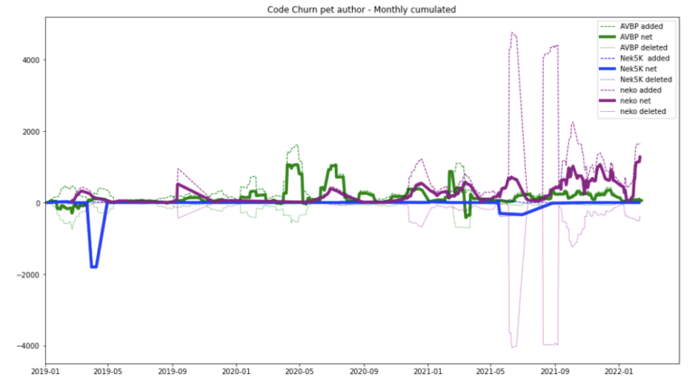
The data is created with git log commands and sorted with code-maat using the abs-churn analysis. Imported in a notebook, the churn is summed over 30 days to make the figure readable. Due to the high number of authors, AVBP churn dwarfs the two others. As the teams are different in size, the same figure is normalized by authors, i.e. AVBP added lines are divided by 115, Nek 5000 by 22, neko by 9.
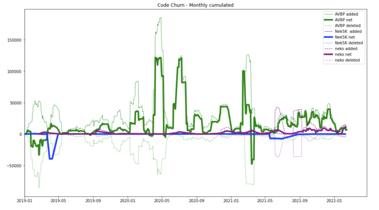
The most striking aspect is how the evolution of AVBP and neko are irregular, with deletions often in sync with additions. An interesting fact about this dataset: for both AVBP and neko, one line is deleted for every 2 lines that are added. Nek5000 is has hardly evolved since 2019, apart from occasional cleaning.
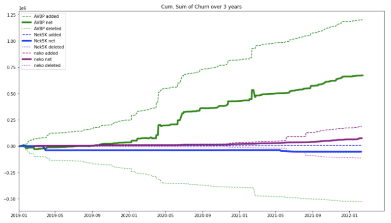
Now if we integrate the absolute churn over time, we see how much each code has grown over three years.
This figure highlights how fast the code is rewritten. On AVBP, a net addition of 10 000 lines per month is possible (which is probably bad news). The AVBP hyper-growth dwarfs the growth of neko
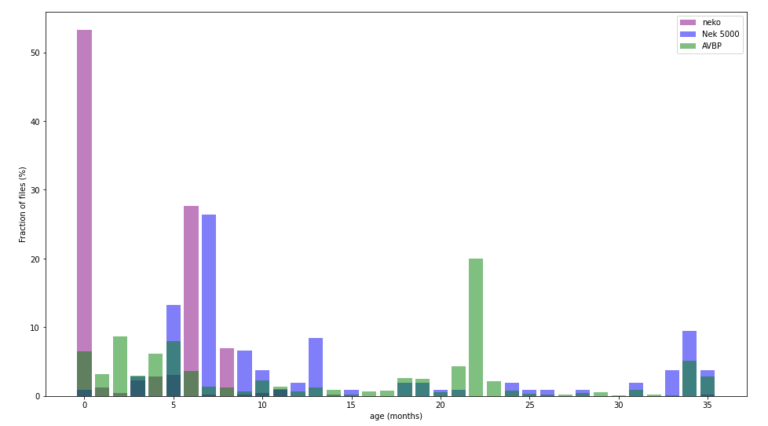
Code age
The next figure is about the age (time since last modification) distribution in each code. According to Tornhill, a good age distribution would be:
- A narrow fraction of the code is very young and actively modified, being the focus of the entire team…
- … and a large fraction of code is aging without the need for support.
For a recent code, you can expect a large fraction of young, frequently modified code. This is well illustrated with the neko codebase. Young codes need time to stabilize. For an abandoned code, young files are rare or inexistent, showing nobody has worked on it.
The AVBP codebase shows three groups. First only 10% of the code is more than three years old, like Nek5000, it is probably hard to keep these codes running on more recent hardware without regular tuning. Then a large refactoring (30%) occurred two years ago, and seems to age quietly. Finally, around 60% of the files have been edited in the last 12 months.
Our last exploration will deal with code complexity. Tornhill points that the number of code lines in a file/function is a good approximation of its complexity.
Regardless of the code’s language, there is a limit to how many new lines a human can process. Opinion varies but this limit is said to be in the range of 50-200 lines. Typically, the popular Python linter pylint issues the too-many-statements when a function/method is over 50 statements.
The next figure shows the numbers of code revisions versus the size in lines for each file.
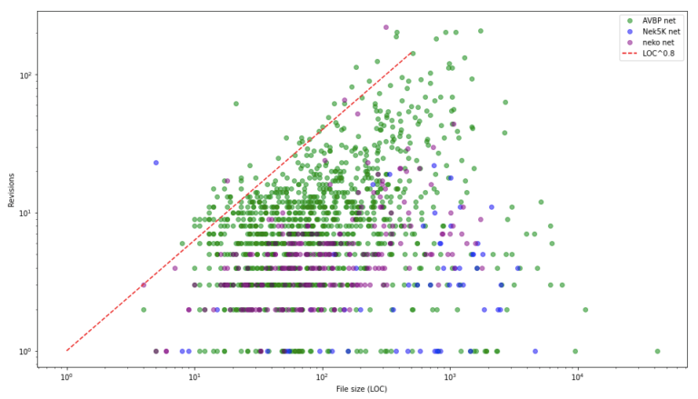
This figure illustrates the general rule that the larger the file, the higher the number of revisions. The files in the upper left corner are obviously interesting candidates for a focused refactoring. More quantitatively, files larger than 1000 lines that have been revised more than 100 times for three years have probably something to tell.
This analysis can even be pushed to the function/subroutine level. Here the tool lizard has been used to scan AVBP and Nek 5000. This tool computes the cyclomatic complexity of code, i.e. the number of paths that can be followed when reading the code. According to Tom McCabe, the interpretation is the following:
- 1-10: simple procedure, little risk
- 11-20: more complex, moderate risk
- 21-50: complex, high risk
- 50+: untestable code, very high risk.
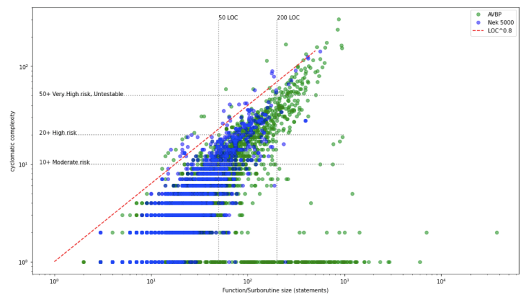
In this last figure, code elements bigger than 200 lines are of high or very high complexity. Almost no code element smaller than 50 lines is high risk.
The whole scatter plot exhibits the same “shark tooth” shape for both codes. It looks like the two independent developers’ communities each respected a similar “acceptable” complexity, roughly below size^0.8 (the red line). Obviously, this trait should be confirmed by comparison with many more HPC CFD repositories.
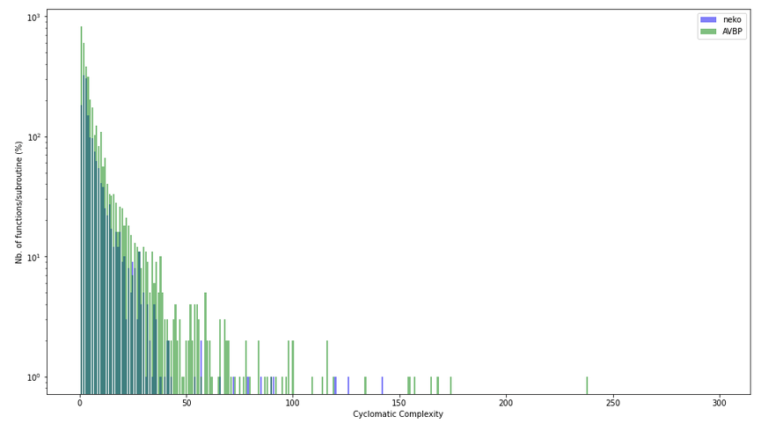
But scatter plots can be misleading because the visual impact of many scattered points does not reflect the actual proportion of points. If we focus only on the distribution of cyclomatic complexity across the functions/subroutine, the most dangerous elements are relatively rare in the code.
|
Cyc. complexity |
AVBP |
Nek 5000 |
|
>20 |
306 (9%) |
100 (6%) |
|
>50 |
74 (2%) |
12/1678 (0.7%) |
Count of high risk and very high-risk files.
Note that in some cases, decreasing the complexity could lead to lower performance: inlining separated functions can be hard for compilers, and high complexity alone does not mean a function must be refactored.
Conclusions
We have applied several codebase analysis techniques inspired by the work of Adam Tornhill to three CFD HPC solvers.
Both code churn and code age illustrate the high level of reworking that has been done. The code churn also showed the fast growth that can occur on active repositories up to 10000 lines of code per month.
The revisions analysis indicates very frequent reworking of the same files, especially the largest ones. Complexity analysis confirmed the presence of numerous examples of highly complex code.
Negatives
- The constant growth, probably powered by the never-ending need to tackle more physically complex situations, could make the code unmanageable in the long run.
- CFD HPC software codebases contain highly complex code.
- In the field of engineering, expertise in modelling and numerics must take precedence over coding experience. The quality of large scientific HPC codes can be reduced when alterations are made by under-experienced developers.
- As each code metric could easily interpreted in two different, and subjective, ways, the figures could fuel useless comparisons and community biases.
- Code metrics should never become goals (see Goodheart law).
Positives
A code metric analysis can give useful insights. Narrowed to only one codebase without comparison, interesting assessments would still emerge such as:
- Our code growth was four times bigger in 2019-22 than in 2015-18. Why this acceleration?
- This highly complex file only required three revisions in the three past years, so it is probably not worth our refactoring time.
- The 10 worst files in the code (high complexity, high revision rates).
- Why some files are highly coupled (often changed at the same time)
- Why these three GPU pragmas are in the MODEL part, while the 12000+ other are in the NUMERICS part.
—Antoine Dauptain, Luis F. Pereìra
Acknowledgements
The authors wish to thank A Tornhill & his team and Terry Yin for bringing these investigative tools to the open source community. A word of gratitude to the decisive action of our former teammate E. “Wonshtrum” Demolis who extended Lizard to Fortran.
This work has been supported by the EXCELLERAT project which has received funding from the European Union’s Horizon 2020 research and innovation program under grant agreement No 823691.